Hello, world: a shakedown of the machinery

Equations, code, a figure, and an interactive growth model — making sure everything on this site works before the real essays start.

This site will carry essays on how frontier AI systems get built — performance engineering on GPUs and TPUs, optimisers for large-batch training, RL and pretraining, the infrastructure underneath — plus occasional pieces on AI’s economics. Before any of that, this post exists to exercise every part of the machinery once.¹ Delete it, or keep it as a colophon.

Equations

Inline math should sit comfortably in a sentence: the arithmetic intensity of a kernel is I = \mathrm{FLOPs} / \mathrm{bytes}, and a kernel is compute-bound when I exceeds the accelerator’s ridge point. Display math should breathe. For a matrix multiply A B with A \in \mathbb{R}^{m \times k}, B \in \mathbb{R}^{k \times n} in half precision (2 bytes per element):

I(m, n, k) \;=\; \frac{2\,mnk}{2\,(mk + kn + mn)} \;=\; \frac{mnk}{mk + kn + mn}.

For square matrices this grows like n/3 — which is why big matmuls are the easiest thing in the world to keep compute-bound, and small ones the hardest.

Code

Syntax highlighting, in the scaling book’s quiet GitHub style:

def arithmetic_intensity(m: int, n: int, k: int, bytes_per_el: int = 2) -> float:
    """FLOPs per byte moved for a naive (no-reuse-in-cache) m*k @ k*n matmul."""
    flops = 2 * m * n * k
    bytes_moved = bytes_per_el * (m * k + k * n + m * n)
    return flops / bytes_moved

# A 4096^3 matmul in fp16 vs. an H100's ~295 FLOP/byte ridge point:
print(f"{arithmetic_intensity(4096, 4096, 4096):.0f} FLOPs/byte")  # ~1365 -> compute-bound

A figure

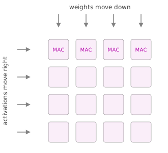
Images and captions:

A 4×4 systolic array, schematically: weights stream down, activations stream right, and each cell does a multiply-accumulate per cycle. The real ones are a little bigger.

An interactive model

The reason this site isn’t on Substack. A Solow-style growth model: capital per worker accumulates as

k_{t+1} = s\,k_t^{\alpha} + (1 - \delta)\,k_t, \qquad k^{*} = \left(\frac{s}{\delta}\right)^{\frac{1}{1-\alpha}},

with output k^\alpha, savings rate s, depreciation \delta, and \alpha = 1/3. Drag the sliders; the trajectory and the steady state k^{*} respond instantly.

viewof s = Inputs.range([0.05, 0.6], {value: 0.3, step: 0.01, label: "Savings rate s"})

viewof delta = Inputs.range([0.02, 0.15], {value: 0.05, step: 0.005, label: "Depreciation δ"})

solow = {
  const alpha = 1 / 3;
  const T = 120;
  let k = 1;
  const path = [{t: 0, k: k}];
  for (let t = 1; t <= T; t++) {
    k = s * Math.pow(k, alpha) + (1 - delta) * k;
    path.push({t: t, k: k});
  }
  return path;
}

kstar = Math.pow(s / delta, 1.5)

Plot.plot({
  width: 660,
  height: 380,
  marginLeft: 50,
  style: {fontSize: "12px"},
  x: {label: "t (periods)"},
  y: {label: "capital per worker, k", grid: true},
  marks: [
    Plot.ruleY([kstar], {stroke: "#b509ac", strokeDasharray: "4 4"}),
    Plot.text([{t: 118, k: kstar}], {
      x: "t", y: "k",
      text: [`k* = ${kstar.toFixed(2)}`],
      dy: -10, fill: "#b509ac", textAnchor: "end", fontWeight: 600
    }),
    Plot.lineY(solow, {x: "t", y: "k", stroke: "#000000", strokeWidth: 1.5})
  ]
})

Later, the same machinery carries anything: a roofline explorer, an attention visualiser, a takeoff model with more dials than anyone needs.

What this post just verified

Inline and display KaTeX; syntax-highlighted code with copy-on-hover; figures with captions; footnotes; category tags on the listing page; and client-side interactive cells with zero server behind them. If you can read this on sombagchi.com with a padlock in the address bar, the pipeline works end to end.

Footnotes

1. Footnotes need testing too.